文章目录

• 单变量线性回归
• • 梯度下降
  • 正则方程
  • 调用sklearn库
• 多变量线性回归

单变量线性回归

导入库

import numpy as np
import pandas as pd
import matplotlib.pyplot as plt

读取数据并展示

#加r保持字符串原始值的含义，即不对其中的符号进行转义
path = r'E:\Master\ML\homework\01 Linear Regression\ex1data1.txt'   
#names添加列名，header用指定的行来作为标题，对无表头的数据，则需设置header=None，否则第一行数据被作为表头
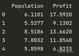
data = pd.read_csv(path,header=None,names=['Population','Profit'])
#head()默认查看前五行，若为-1，则查看至倒数第二行
data.head()
print(data.head())
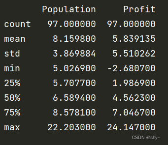
#describe()快速统计汇总数据内容
data.describe()   
print(data.describe())

绘制散点图，可视化理解数据

data.plot(kind='scatter',x='Population',y='Profit',figsize=(8,5))
plt.show()

数据预处理
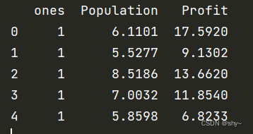
为了使用向量化的方式计算代价函数和梯度，首先在训练集中添加一列

data.insert(0,'ones',1)
print(data.head())

添加一列后的数据如图示

接着对变量进行初始化，取最后一列为y，其余为X

#shape()读取矩阵的长度
#使用shape[0]读取矩阵第一维度的长度，即行数；使用shape[1]读取矩阵第二维度的长度，即列数
cols = data.shape[1]    #列数
#iloc[]函数对数据进行位置索引，从而在数据表中提取出相应的数据
#iloc[a:b,c:d]:取行索引从a到b-1，列索引从c到d-1的数据，左到右不到
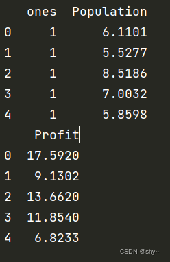
X = data.iloc[:,0:cols-1]   #取前cols-1列作为输入向量
y = data.iloc[:,cols-1:cols] #取最后一列作为目标向量
#观察训练集和目标变量是否正确
print(X.head())
print(y.head())
X = np.matrix(X.values)
y = np.matrix(y.values)
theta = np.matrix([0,0])

查看维度，确保没问题

print(X.shape)
print(y.shape)
print(theta.shape)

定义代价函数

#power(a,b)若b为单个数字，则对a各个元素分别求b次方
#若b为数组，其列数要与a相同，并求相应的次方
def computeCost(X,y,theta):inner = np.power(((X*theta.T)-y),2)return np.sum(inner)/(2*len(X))#计算初始代价函数的值
computeCost(X,y,theta)
print(computeCost(X,y,theta))

梯度下降

def gradientDescent(X,y,theta,alpha,epoch):temp = np.matrix(np.zeros(theta.shape))      #初始化一个θ临时矩阵（1，2）# flatten()即返回一个折叠成一维的数组parameters = int(theta.flatten().shape[1])    #参数θ的数量cost = np.zeros(epoch)   #初始化一个ndarrsy，包含每次训练后的costm = X.shape[0]     #样本数量mfor i in range(epoch):temp =theta - (alpha / m) * (X * theta.T - y).T * Xtheta = tempcost[i] = computeCost(X,y,theta)return theta,cost

初始化一些附加变量 - 学习率α和要执行的迭代次数

alpha = 0.01
epoch = 1000

运行梯度下降

final_theta,cost = gradientDescent(X,y,theta,alpha,epoch)
#使用拟合的参数计算cost
computeCost(X,y,final_theta)
print(computeCost(X,y,final_theta))

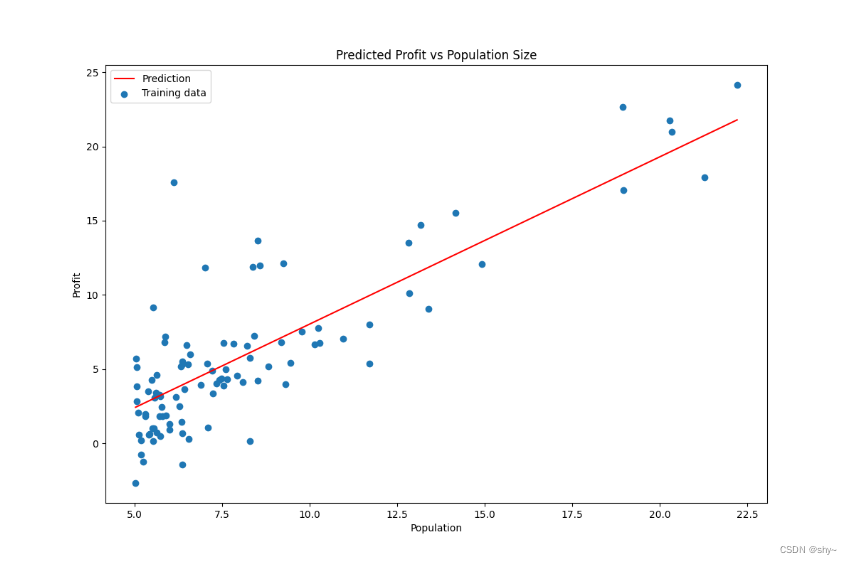
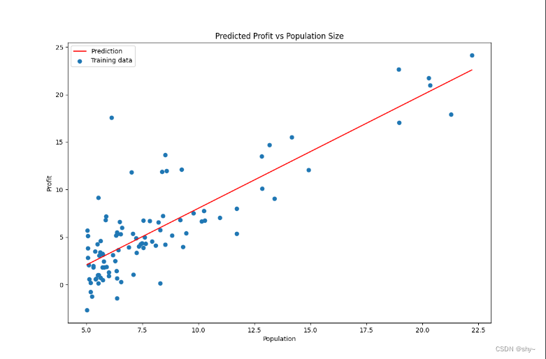
绘制数据拟合图

#np.linspace()在指定的间隔内返回均匀间隔的数字
#np.linspace(start = , stop = , num = )
x = np.linspace(data.Population.min(),data.Population.max(),100)   #横坐标
f = final_theta[0,0] + (final_theta[0,1] * x)     #纵坐标，利润#画出数据拟合图
#fig：画布对象 ax：坐标系子图对象或者轴对象的数组
fig1,ax = plt.subplots(figsize=(12,8))     #如果只创建了一个子图像，返回的坐标轴对象是一个标量，可以直接引用
ax.plot(x,f,label='Prediction',color='red')
ax.scatter(data['Population'],data.Profit,label='Training data')
ax.legend(loc=2)   #2表示在左上角
ax.set_xlabel('Population')
ax.set_ylabel('Profit')
ax.set_title('Predicted Profit vs Population Size')
plt.show()

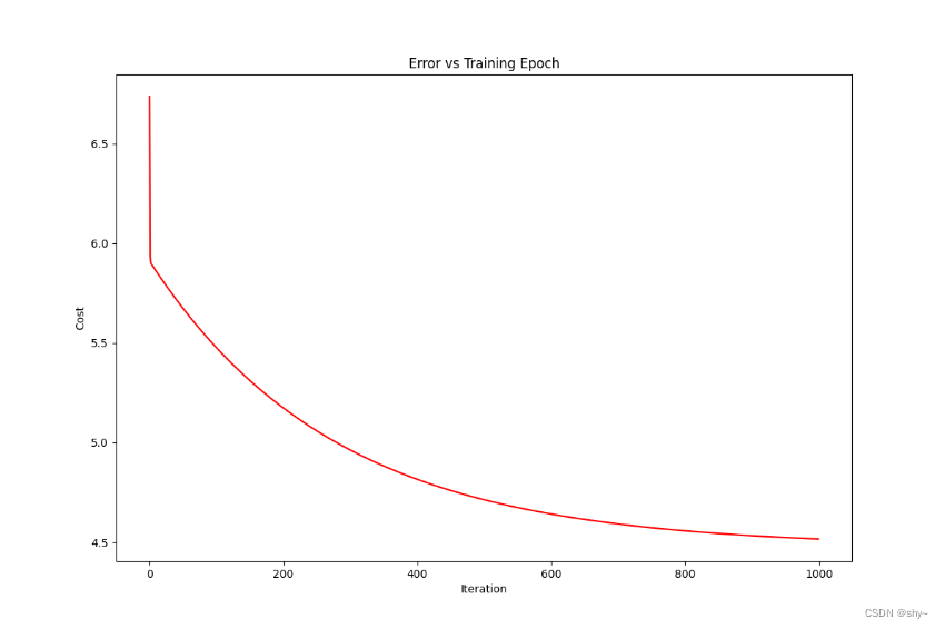
绘制损失函数图

fig, ax = plt.subplots(figsize=(12,8))
ax.plot(np.arange(epoch),cost,'r')    #np.arange返回等差数组
ax.set_xlabel('Iteration')
ax.set_ylabel('Cost')
ax.set_title('Error vs Training Epoch')
plt.show()

正则方程

在特征数不那么多的情况下，使用正则方程可以达到跟梯度下降一样的效果

#定义正则方程
def normalEqn(X,y):
#numpy.linalg模块包含线性代数的函数。使用这个模块，可以计算逆矩阵、求特征值、解线性方程组以及求解行列式等theta = np.linalg.inv(X.T@X)@X.T@yreturn thetatheta = normalEqn(X,y)
#print(theta)computeCost(X,y,theta.reshape(1,-1))   #将θ变成一行
#print(computeCost(X,y,theta.reshape(1,-1)))#画出拟合图像
x = np.linspace(data['Population'].min(),data.Population.max(),100)
f = theta[0,0] + theta[1,0]*xplt.figure(figsize=(12,8))
plt.xlabel('Population')
plt.ylabel('Profit')
l1 = plt.plot(x,f,label='Prediction',color='red')
l2 = plt.scatter(data.Population,data.Profit,label='Training data')
plt.legend(loc='best')
plt.title('Predicted Profit vs Population Size')
plt.show()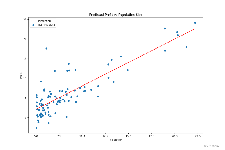

调用sklearn库

sklearn是一个非常著名的机器学习库，广泛地用于统计分析和机器学习建模等数据科学领域。

from sklearn import linear_model
#linear_model.LinearRegression(fit_intercept=True,copy_X=True,n_jobs=-1,positive=False)
#fit_intercept bool值，只支持true/false  模型是否拟合截距项，默认为true
#copy_x bool值，只支持true/false 特征矩阵X是否需要拷贝，默认为true,scikit-learn做的运算不会影响原始数据，否则矩阵X可能被覆盖
#n_jobs  int型 使用多少个processor完成这个拟合任务，默认为None（也就是1）
#positive bool型 是否限制拟合的系数为正数，默认为false
model = linear_model.LinearRegression()      #建立线性回归对象
model.fit(np.array(X),np.array(y))
#print(X[:,1].A1.shape)x = np.array(X[:,1].A1)                 #取第二列，转换成一维的
f = model.predict(np.array(X)).flatten()          #预测之后也转换成一维的#画出数据拟合图
fig,ax = plt.subplots(figsize=(12,8))
ax.plot(x,f,'r',label='Prediction')
ax.scatter(data.Population,data.Profit,label='Training Data')
ax.legend(loc=2)   #左上角
ax.set_xlabel('Population')
ax.set_ylabel('Profit')
ax.set_title('Predicted Profit vs Population Szie')
plt.show()

多变量线性回归

导入库、读取数据并展示 同单变量线性回归，不再赘述
特征缩放
不同特征的取值范围差别较大，为了使梯度下降更快收敛，对特征进行归一化处理

#保存means、std、mins、maxs、data
means = data.mean().values
stds = data.std().values
mins = data.min().values
maxs = data.max().values
data_ = data.values
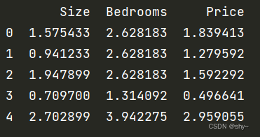
data.describe()#特征缩放
data = (data - mins)/stds
data.head()
print(data.head())

数据预处理

data.insert(0,'ones',1)
#print(data.head())cols = data.shape[1]      #列数
X = data.iloc[:,:cols-1]   #取前cols-1列作为输入向量
y = data.iloc[:,cols-1:cols]  #取最后一列作为目标向量
#print(y.head())X = np.matrix(X.values)
y = np.matrix(y.values)
theta = np.matrix(np.array([0,0,0]))
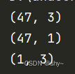
#查看维度，确认是否正确
print(X.shape)
print(y.shape)
print(theta.shape)

定义损失函数

#定义损失函数
def computeCost(X,y,theta):inner = np.power(((X*theta.T)-y),2)return np.sum(inner)/(2*len(X))

定义梯度下降

#定义梯度下降函数
def gradientDescent(X,y,theta,alpha,epoch):temp = np.matrix(np.zeros(theta.shape))      #初始化一个θ临时矩阵（1，3）parameters = int(theta.flatten().shape[1])cost = np.zeros(epoch)m = X.shape[0]             #样本数量mfor i in range(epoch):temp = theta - (alpha/m)*(X*theta.T-y).T*Xtheta = tempcost[i] = computeCost(X,y,theta)return theta,costalpha = 0.01
epoch = 1000#运行梯度下降算法
final_theta,cost = gradientDescent(X,y,theta,alpha,epoch)

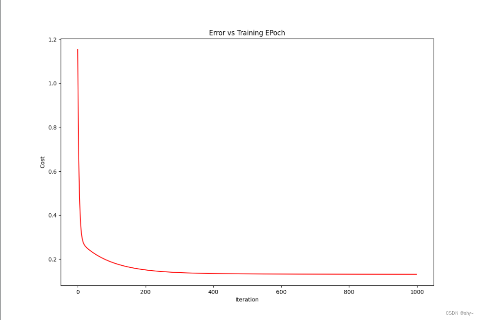
损失函数图

fig1, ax = plt.subplots(figsize=(12,8))
ax.plot(np.arange(epoch),cost,'r')
ax.set_xlabel('Iteration')
ax.set_ylabel('Cost')
ax.set_title('Error vs Training EPoch')
plt.show()

价格预测

#参数转化为缩放前
def theta_transform(theta, means, stds):temp = means[:-1] * theta[1:] / stds[:-1]theta[0] = (theta[0] - np.sum(temp)) * stds[-1] + means[-1]theta[1:] = theta[1:] * stds[-1] / stds[:-1]return theta.reshape(1, -1)g_ = np.array(final_theta.reshape(-1, 1))
means = means.reshape(-1, 1)
stds = stds.reshape(-1, 1)
transform_g = theta_transform(g_, means, stds)
#print(transform_g)# 预测价格
def predictPrice(x, y, theta):return theta[0, 0] + theta[0, 1]*x + theta[0, 2]*y# 2104,3,399900,
price = predictPrice(2104, 3, transform_g)
print(price)

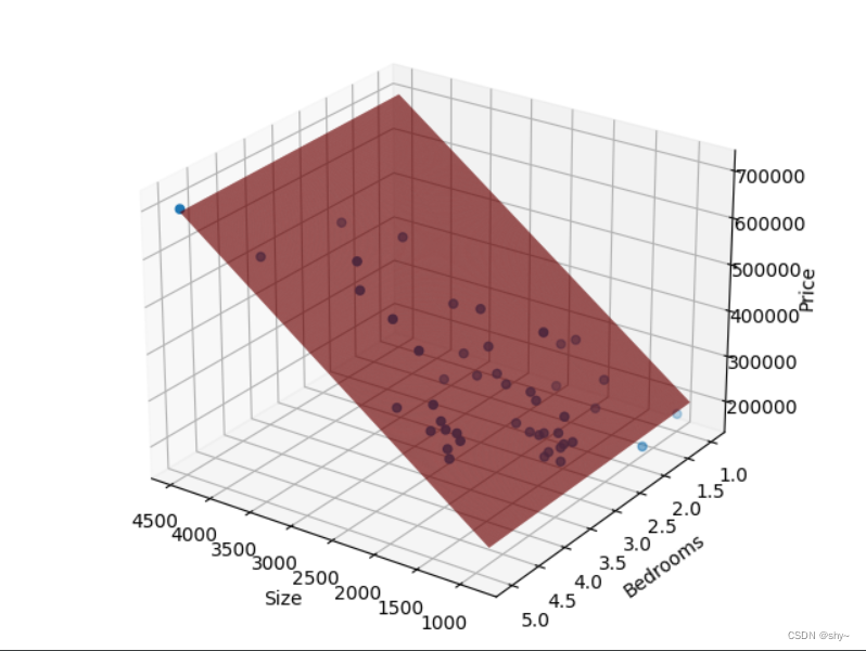
平面拟合图

from mpl_toolkits.mplot3d import Axes3D
fig = plt.figure()
ax = Axes3D(fig)
X_ = np.arange(mins[0], maxs[0]+1, 1)
Y_ = np.arange(mins[1], maxs[1]+1, 1)
X_, Y_ = np.meshgrid(X_, Y_)
Z_ = transform_g[0,0] + transform_g[0,1] * X_ + transform_g[0,2] * Y_# 手动设置角度
ax.view_init(elev=25, azim=125)ax.set_xlabel('Size')
ax.set_ylabel('Bedrooms')
ax.set_zlabel('Price')ax.plot_surface(X_, Y_, Z_, rstride=1, cstride=1, color='red')ax.scatter(data_[:, 0], data_[:, 1], data_[:, 2])
plt.show()

当作对自己学习的记录，后面还有部分代码不是很懂，欢迎大家一起交流学习~